[Wang and Dowling, 2022] Wang, Jialu, and Alexander W. Dowling.
“Pyomo.DOE: An open‐source package for model‐based design of experiments in Python.”
AIChE Journal 68.12 (2022): e17813. https://doi.org/10.1002/aic.17813
Methodology Overview
Model-based Design of Experiments (MBDoE) is a technique to maximize the information
gain from experiments by directly using science-based models with physically meaningful
parameters. It is one key component in the model calibration and uncertainty
quantification workflow shown below:
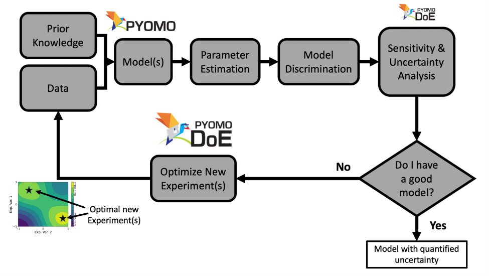
The parameter estimation, uncertainty analysis, and MBDoE are
combined into an iterative framework to select, refine, and calibrate science-based
mathematical models with quantified uncertainty. Currently, Pyomo.DoE focuses on
increasing parameter precision.
Pyomo.DoE provides the exploratory analysis and MBDoE capabilities to the
Pyomo ecosystem. The user provides one Pyomo model, a set of parameter nominal values,
the allowable design spaces for design variables, and the assumed observation error model.
During exploratory analysis, Pyomo.DoE checks if the model parameters can be
inferred from the postulated measurements or preliminary data.
MBDoE then recommends optimized experimental conditions for collecting more data.
Parameter estimation packages such as Parmest can perform
parameter estimation using the available data to infer values for parameters,
and facilitate an uncertainty analysis to approximate the parameter covariance matrix.
If the parameter uncertainties are sufficiently small, the workflow terminates
and returns the final model with quantified parametric uncertainty.
If not, MBDoE recommends optimized experimental conditions to generate new data
that will maximize information gain and eventually reduce parameter uncertainty.
Below is an overview of the type of optimization models Pyomo.DoE can accommodate:
Pyomo.DoE is suitable for optimization models of continuous variables
Pyomo.DoE can handle equality constraints defining state variables
Pyomo.DoE supports (Partial) Differential-Algebraic Equations (PDAE) models via Pyomo.DAE
Pyomo.DoE also supports models with only algebraic equations
The general form of a DAE problem that can be passed into Pyomo.DoE is shown below:
\[\begin{array}{l}
\dot{\mathbf{x}}(t) = \mathbf{f}(\mathbf{x}(t), \mathbf{z}(t), \mathbf{y}(t), \mathbf{u}(t), \overline{\mathbf{w}}, \boldsymbol{\theta}) \\
\mathbf{g}(\mathbf{x}(t), \mathbf{z}(t), \mathbf{y}(t), \mathbf{u}(t), \overline{\mathbf{w}},\boldsymbol{\theta})=\mathbf{0} \\
\mathbf{y} =\mathbf{h}(\mathbf{x}(t), \mathbf{z}(t), \mathbf{u}(t), \overline{\mathbf{w}},\boldsymbol{\theta}) \\
\mathbf{f}^{\mathbf{0}}\left(\dot{\mathbf{x}}\left(t_{0}\right), \mathbf{x}\left(t_{0}\right), \mathbf{z}(t_0), \mathbf{y}(t_0), \mathbf{u}\left(t_{0}\right), \overline{\mathbf{w}}, \boldsymbol{\theta}\right)=\mathbf{0} \\
\mathbf{g}^{\mathbf{0}}\left( \mathbf{x}\left(t_{0}\right),\mathbf{z}(t_0), \mathbf{y}(t_0), \mathbf{u}\left(t_{0}\right), \overline{\mathbf{w}}, \boldsymbol{\theta}\right)=\mathbf{0}\\
\mathbf{y}^{\mathbf{0}}\left(t_{0}\right)=\mathbf{h}\left(\mathbf{x}\left(t_{0}\right),\mathbf{z}(t_0), \mathbf{u}\left(t_{0}\right), \overline{\mathbf{w}}, \boldsymbol{\theta}\right)
\end{array}\]
where:
\(\boldsymbol{\theta} \in \mathbb{R}^{N_p}\) are unknown model parameters.
\(\mathbf{x} \subseteq \mathcal{X}\) are dynamic state variables which characterize trajectory of the system, \(\mathcal{X} \in \mathbb{R}^{N_x \times N_t}\).
\(\mathbf{z} \subseteq \mathcal{Z}\) are algebraic state variables, \(\mathcal{Z} \in \mathbb{R}^{N_z \times N_t}\).
\(\mathbf{u} \subseteq \mathcal{U}\) are time-varying decision variables, \(\mathcal{U} \in \mathbb{R}^{N_u \times N_t}\).
\(\overline{\mathbf{w}} \in \mathbb{R}^{N_w}\) are time-invariant decision variables.
\(\mathbf{y} \subseteq \mathcal{Y}\) are measurement response variables, \(\mathcal{Y} \in \mathbb{R}^{N_r \times N_t}\).
\(\mathbf{f}(\cdot)\) are differential equations.
\(\mathbf{g}(\cdot)\) are algebraic equations.
\(\mathbf{h}(\cdot)\) are measurement functions.
\(\mathbf{t} \in \mathbb{R}^{N_t \times 1}\) is a union of all time sets.
Note
Parameters and design variables should be defined as Pyomo Var components
when building the model using the Experiment class so that users can use both
Parmest and Pyomo.DoE seamlessly.
Based on the above notation, the form of the MBDoE problem addressed in Pyomo.DoE is shown below:
\begin{equation}
\begin{aligned}
\underset{\boldsymbol{\varphi}}{\max} \quad & \Psi (\mathbf{M}(\boldsymbol{\hat{\theta}}, \boldsymbol{\varphi})) \\
\text{s.t.} \quad & \mathbf{M}(\boldsymbol{\hat{\theta}}, \boldsymbol{\varphi}) = \sum_r^{N_r} \sum_{r'}^{N_r} \tilde{\sigma}_{(r,r')}\mathbf{Q}_r^\mathbf{T} \mathbf{Q}_{r'} + \mathbf{M}_0 \\
& \dot{\mathbf{x}}(t) = \mathbf{f}(\mathbf{x}(t), \mathbf{z}(t), \mathbf{y}(t), \mathbf{u}(t), \overline{\mathbf{w}}, \boldsymbol{\hat{\theta}}) \\
& \mathbf{g}(\mathbf{x}(t), \mathbf{z}(t), \mathbf{y}(t), \mathbf{u}(t), \overline{\mathbf{w}},\boldsymbol{\hat{\theta}})=\mathbf{0} \\
& \mathbf{y} =\mathbf{h}(\mathbf{x}(t), \mathbf{z}(t), \mathbf{u}(t), \overline{\mathbf{w}},\boldsymbol{\hat{\theta}}) \\
& \mathbf{f}^{\mathbf{0}}\left(\dot{\mathbf{x}}\left(t_{0}\right), \mathbf{x}\left(t_{0}\right), \mathbf{z}(t_0), \mathbf{y}(t_0), \mathbf{u}\left(t_{0}\right), \overline{\mathbf{w}}, \boldsymbol{\hat{\theta}})\right)=\mathbf{0} \\
& \mathbf{g}^{\mathbf{0}}\left( \mathbf{x}\left(t_{0}\right),\mathbf{z}(t_0), \mathbf{y}(t_0), \mathbf{u}\left(t_{0}\right), \overline{\mathbf{w}}, \boldsymbol{\hat{\theta}}\right)=\mathbf{0}\\
&\mathbf{y}^{\mathbf{0}}\left(t_{0}\right)=\mathbf{h}\left(\mathbf{x}\left(t_{0}\right),\mathbf{z}(t_0), \mathbf{u}\left(t_{0}\right), \overline{\mathbf{w}}, \boldsymbol{\hat{\theta}}\right)
\end{aligned}
\end{equation}
where:
\(\boldsymbol{\varphi}\) are design variables, which are manipulated to maximize the information content of experiments. It should consist of one or more of \(\mathbf{u}(t), \mathbf{y}^{\mathbf{0}}({t_0}),\overline{\mathbf{w}}\). With a proper model formulation, the timepoints for control or measurements \(\mathbf{t}\) can also be degrees of freedom.
\(\mathbf{M}\) is the Fisher information matrix (FIM), approximated as the inverse of the covariance matrix of parameter estimates \(\boldsymbol{\hat{\theta}}\). A large FIM indicates more information contained in the experiment for parameter estimation.
\(\mathbf{Q}\) is the dynamic sensitivity matrix, containing the partial derivatives of \(\mathbf{y}\) with respect to \(\boldsymbol{\theta}\).
\(\Psi\) is the scalar design criteria to measure the information content in the FIM.
\(\mathbf{M}_0\) is the sum of all the FIMs from previous experiments.
Pyomo.DoE provides five design criteria \(\Psi\) to measure the information in the FIM.
The covariance matrix of parameter estimates is approximated as the inverse of the FIM,
i.e., \(\mathbf{V} \approx \mathbf{M}^{-1}\).
We can use the FIM or the covariance matrix to define the design criteria.
Table 5 Pyomo.DoE design criteria
Design criterion |
Computation |
Geometrical meaning |
|---|
A-optimality |
\(\text{trace}(\mathbf{V}) = \text{trace}(\mathbf{M}^{-1})\) |
Minimizing this is equivalent to minimizing the enclosing box of the confidence ellipse |
Pseudo A-optimality |
\(\text{trace}(\mathbf{M})\) |
Maximizing this is equivalent to maximizing the dimensions of the enclosing box of the Fisher Information Matrix |
D-optimality |
\(\det(\mathbf{M}) = 1/\det(\mathbf{V})\) |
Maximizing this is equivalent to minimizing confidence-ellipsoid volume |
E-optimality |
\(\lambda_{\min}(\mathbf{M}) = 1/\lambda_{\max}(\mathbf{V})\) |
Maximizing this is equivalent to minimizing the longest axis of the confidence ellipse |
Modified E-optimality |
\(\text{cond}(\mathbf{M}) = \text{cond}(\mathbf{V})\) |
Minimizing this is equivalent to minimizing the ratio of the longest axis to the shortest axis of the confidence ellipse |
Note
A confidence ellipse is a geometric representation of the uncertainty in parameter
estimates. It is derived from the covariance matrix \(\mathbf{V}\).
In order to solve problems of the above, Pyomo.DoE implements the 2-stage stochastic program. Please see Wang and Dowling (2022) for details.
Pyomo.DoE Usage Example
We illustrate the use of Pyomo.DoE using a reaction kinetics example (Wang and Dowling, 2022).
\begin{equation}
A \xrightarrow{k_1} B \xrightarrow{k_2} C
\end{equation}
The Arrhenius equations model the temperature dependence of the reaction rate coefficients \(k_1\) and \(k_2\). Assuming a first-order reaction mechanism gives the reaction rate model shown below. Further, we assume only species A is fed to the reactor.
\begin{equation}
\begin{aligned}
k_1 & = A_1 e^{-\frac{E_1}{RT}} \\
k_2 & = A_2 e^{-\frac{E_2}{RT}} \\
\frac{d{C_A}}{dt} & = -k_1{C_A} \\
\frac{d{C_B}}{dt} & = k_1{C_A} - k_2{C_B} \\
C_{A0}& = C_A + C_B + C_C \\
C_B(t_0) & = 0 \\
C_C(t_0) & = 0 \\
\end{aligned}
\end{equation}
\(C_A(t), C_B(t), C_C(t)\) are the time-varying concentrations of the species A, B, C, respectively.
\(k_1, k_2\) are the rate constants for the two chemical reactions using an Arrhenius equation with activation energies \(E_1, E_2\) and pre-exponential factors \(A_1, A_2\).
The goal of MBDoE is to optimize the experiment design variables \(\boldsymbol{\varphi} = (C_{A0}, T(t))\), where \(C_{A0},T(t)\) are the initial concentration of species A and the time-varying reactor temperature, to maximize the precision of unknown model parameters \(\boldsymbol{\theta} = (A_1, E_1, A_2, E_2)\) by measuring \(\mathbf{y}(t)=(C_A(t), C_B(t), C_C(t))\).
The observation errors are assumed to be independent both in time and across measurements with a constant standard deviation of 1 M for each species.
Step 0: Import Pyomo and the Pyomo.DoE module and create an Experiment class
Note
This example uses the data file result.json, located in the Pyomo repository at:
pyomo/contrib/doe/examples/result.json, which contains the nominal parameter
values, and measurements for the reaction kinetics experiment.
import pyomo.environ as pyo
from pyomo.dae import ContinuousSet, DerivativeVar, Simulator
from pyomo.contrib.parmest.experiment import Experiment
Subclass the Parmest Experiment class to define the reaction
kinetics experiment and build the Pyomo ConcreteModel.
class ReactorExperiment(Experiment):
    def __init__(self, data, nfe, ncp):
        """
        Arguments
        ---------
        data: object containing vital experimental information
        nfe: number of finite elements
        ncp: number of collocation points for the finite elements
        """
        self.data = data
        self.nfe = nfe
        self.ncp = ncp
        self.model = None

        #############################
Step 1: Define the Pyomo process model
The process model for the reaction kinetics problem is shown below. Here, we build
the model without any data or discretization.
    def create_model(self):
        """
        This is an example user model provided to DoE library.
        It is a dynamic problem solved by Pyomo.DAE.

        Return
        ------
        m: a Pyomo.DAE model
        """

        m = self.model = pyo.ConcreteModel()

        # Model parameters
        m.R = pyo.Param(mutable=False, initialize=8.314)

        # Define model variables
        ########################
        # time
        m.t = ContinuousSet(bounds=[0, 1])

        # Concentrations
        m.CA = pyo.Var(m.t, within=pyo.NonNegativeReals)
        m.CB = pyo.Var(m.t, within=pyo.NonNegativeReals)
        m.CC = pyo.Var(m.t, within=pyo.NonNegativeReals)

        # Temperature
        m.T = pyo.Var(m.t, within=pyo.NonNegativeReals)

        # Arrhenius rate law equations
        m.A1 = pyo.Var(within=pyo.NonNegativeReals)
        m.E1 = pyo.Var(within=pyo.NonNegativeReals)
        m.A2 = pyo.Var(within=pyo.NonNegativeReals)
        m.E2 = pyo.Var(within=pyo.NonNegativeReals)

        # Differential variables (Conc.)
        m.dCAdt = DerivativeVar(m.CA, wrt=m.t)
        m.dCBdt = DerivativeVar(m.CB, wrt=m.t)

        ########################
        # End variable def.

        # Equation definition
        ########################

        # Expression for rate constants
        @m.Expression(m.t)
        def k1(m, t):
            return m.A1 * pyo.exp(-m.E1 * 1000 / (m.R * m.T[t]))

        @m.Expression(m.t)
        def k2(m, t):
            return m.A2 * pyo.exp(-m.E2 * 1000 / (m.R * m.T[t]))

        # Concentration odes
        @m.Constraint(m.t)
        def CA_rxn_ode(m, t):
            return m.dCAdt[t] == -m.k1[t] * m.CA[t]

        @m.Constraint(m.t)
        def CB_rxn_ode(m, t):
            return m.dCBdt[t] == m.k1[t] * m.CA[t] - m.k2[t] * m.CB[t]

        # algebraic balance for concentration of C
        # Valid because the reaction system (A --> B --> C) is equimolar
        @m.Constraint(m.t)
        def CC_balance(m, t):
            return m.CA[0] == m.CA[t] + m.CB[t] + m.CC[t]

        ########################
Step 2: Finalize the Pyomo process model
Here, we add data to the model and finalize the discretization using a new method to
the class. This step is required before the model can be labeled.
    def finalize_model(self):
        """
        Example finalize model function. There are two main tasks
        here:

            1. Extracting useful information for the model to align
               with the experiment. (Here: CA0, t_final, t_control)
            2. Discretizing the model subject to this information.

        """
        m = self.model

        # Unpacking data before simulation
        control_points = self.data["control_points"]

        # Set initial concentration values for the experiment
        m.CA[0].value = self.data["CA0"]
        m.CB[0].fix(self.data["CB0"])

        # Update model time `t` with time range and control time points
        m.t.update(self.data["t_range"])
        m.t.update(control_points)

        # Fix the unknown parameter values
        m.A1.fix(self.data["A1"])
        m.A2.fix(self.data["A2"])
        m.E1.fix(self.data["E1"])
        m.E2.fix(self.data["E2"])

        # Add upper and lower bounds to the design variable, CA[0]
        m.CA[0].setlb(self.data["CA_bounds"][0])
        m.CA[0].setub(self.data["CA_bounds"][1])

        m.t_control = control_points

        # Discretizing the model
        discr = pyo.TransformationFactory("dae.collocation")
        discr.apply_to(m, nfe=self.nfe, ncp=self.ncp, wrt=m.t)

        # Initializing Temperature in the model
        cv = None
        for t in m.t:
            if t in control_points:
                cv = control_points[t]
                m.T[t].fix()
            m.T[t].setlb(self.data["T_bounds"][0])
            m.T[t].setub(self.data["T_bounds"][1])
            m.T[t] = cv

        # Make a constraint that holds temperature constant between control time points
        @m.Constraint(m.t - control_points)
        def T_control(m, t):
            """
            Piecewise constant temperature between control points
            """
            neighbour_t = max(tc for tc in control_points if tc < t)
            return m.T[t] == m.T[neighbour_t]

        #########################
Step 4: Implement the get_labeled_model method
This method utilizes the previous 3 steps and is used by Pyomo.DoE to build the model
to perform optimal experimental design.
    def get_labeled_model(self):
        if self.model is None:
            self.create_model()
            self.finalize_model()
            self.label_experiment()
        return self.model
Step 5: Exploratory analysis (Enumeration)
After creating the subclass of the Experiment class, exploratory analysis is
suggested to enumerate the design space to check if the problem is identifiable,
i.e., ensure that D-, E-optimality metrics are not small numbers near zero, and
Modified E-optimality is not a big number.
Additionally, it helps to initialize the model for the optimal experimental design step.
Pyomo.DoE can perform exploratory sensitivity analysis with the compute_FIM_full_factorial method.
The compute_FIM_full_factorial method generates a grid over the design space as specified by the user.
Each grid point represents an MBDoE problem solved using the compute_FIM method.
In this way, sensitivity of the FIM over the design space can be evaluated.
Pyomo.DoE supports plotting the results from the compute_FIM_full_factorial method
with the draw_factorial_figure method.
The following code defines the run_reactor_doe function. This function encapsulates
the workflow for both sensitivity analysis (Step 5) and optimal design (Step 6).
from pyomo.common.dependencies import numpy as np, pathlib

from pyomo.contrib.doe.examples.reactor_experiment import ReactorExperiment
from pyomo.contrib.doe import DesignOfExperiments

import pyomo.environ as pyo

import json


# Example for sensitivity analysis on the reactor experiment
# After sensitivity analysis is done, we perform optimal DoE
def run_reactor_doe(
    n_points_for_C0: int = 9,
    n_points_for_T0: int = 9,
    C0_bounds_for_factorial: tuple = (1, 5),
    T0_bounds_for_factorial: tuple = (300, 700),
    compute_FIM_full_factorial=True,
    plot_factorial_results=True,
    figure_file_name="example_reactor_compute_FIM",
    log_scale=False,
    run_optimal_doe=True,
):
    """
    This function demonstrates how to perform sensitivity analysis on the reactor

    Parameters
    ----------
    n_points_for_C0 : int, optional
        number of points to use for the C0 design range, by default 9
    n_points_for_T0 : int, optional
        number of points to use for the T0 design range, by default 9
    compute_FIM_full_factorial : bool, optional
        whether to compute the full factorial design, by default True
    plot_factorial_results : bool, optional
        whether to plot the results of the full factorial design, by default True
    figure_file_name : str, optional
        file name to save the factorial figure, by default "example_reactor_compute_FIM"
    run_optimal_doe : bool, optional
        whether to run the optimal DoE, by default True
    """
    # Read in file
    DATA_DIR = pathlib.Path(__file__).parent
    file_path = DATA_DIR / "result.json"

    with open(file_path) as f:
        data_ex = json.load(f)

    # Put temperature control time points into correct format for reactor experiment
    data_ex["control_points"] = {
        float(k): v for k, v in data_ex["control_points"].items()
    }

    # Create a ReactorExperiment object; data and discretization information are part
    # of the constructor of this object
    experiment = ReactorExperiment(data=data_ex, nfe=10, ncp=3)

    # Use a central difference, with step size 1e-3
    fd_formula = "central"
    step_size = 1e-3

    # Use the determinant objective with scaled sensitivity matrix
    objective_option = "determinant"
    scale_nominal_param_value = True

    # Create the DesignOfExperiments object
    # We will not be passing any prior information in this example
    # and allow the experiment object and the DesignOfExperiments
    # call of ``run_doe`` perform model initialization.
    doe_obj = DesignOfExperiments(
        experiment,
        fd_formula=fd_formula,
        step=step_size,
        objective_option=objective_option,
        scale_constant_value=1,
        scale_nominal_param_value=scale_nominal_param_value,
        prior_FIM=None,
        jac_initial=None,
        fim_initial=None,
        L_diagonal_lower_bound=1e-7,
        solver=None,
        tee=False,
        get_labeled_model_args=None,
        _Cholesky_option=True,
        _only_compute_fim_lower=True,
    )
    if compute_FIM_full_factorial:
        # Make design ranges to compute the full factorial design
        design_ranges = {
            "CA[0]": [*C0_bounds_for_factorial, n_points_for_C0],
            "T[0]": [*T0_bounds_for_factorial, n_points_for_T0],
        }

        # Compute the full factorial design with the sequential FIM calculation
        doe_obj.compute_FIM_full_factorial(
            design_ranges=design_ranges, method="sequential"
        )
    if plot_factorial_results:
        # Plot the results
        doe_obj.draw_factorial_figure(
            sensitivity_design_variables=["CA[0]", "T[0]"],
            fixed_design_variables={
                "T[0.125]": 300,
                "T[0.25]": 300,
                "T[0.375]": 300,
                "T[0.5]": 300,
                "T[0.625]": 300,
                "T[0.75]": 300,
                "T[0.875]": 300,
                "T[1]": 300,
            },
            title_text="Reactor Example",
            xlabel_text="Concentration of A (M)",
            ylabel_text="Initial Temperature (K)",
            figure_file_name=figure_file_name,
            log_scale=log_scale,
        )

    ###########################
    # End sensitivity analysis

    # Begin optimal DoE
    ####################
    if run_optimal_doe:
        doe_obj.run_doe()

        # Print out a results summary
        print("Optimal experiment values: ")
        print(
            "\tInitial concentration: {:.2f}".format(
                doe_obj.results["Experiment Design"][0]
            )
        )
        print(
            ("\tTemperature values: [" + "{:.2f}, " * 8 + "{:.2f}]").format(
                *doe_obj.results["Experiment Design"][1:]
            )
        )
        print("FIM at optimal design:\n {}".format(np.array(doe_obj.results["FIM"])))
        print(
            "Objective value at optimal design: {:.2f}".format(
                pyo.value(doe_obj.model.objective)
            )
        )

        print(doe_obj.results["Experiment Design Names"])

        ###################
        # End optimal DoE

    return doe_obj
After defining the function, we will call it to perform the exploratory analysis and
the optimal experimental design.
run_reactor_doe(figure_file_name=None)
A design exploration for the initial concentration and temperature as experimental
design variables with 9 values for each, produces the the five figures for
five optimality criteria using the compute_FIM_full_factorial and
draw_factorial_figure methods as shown below:
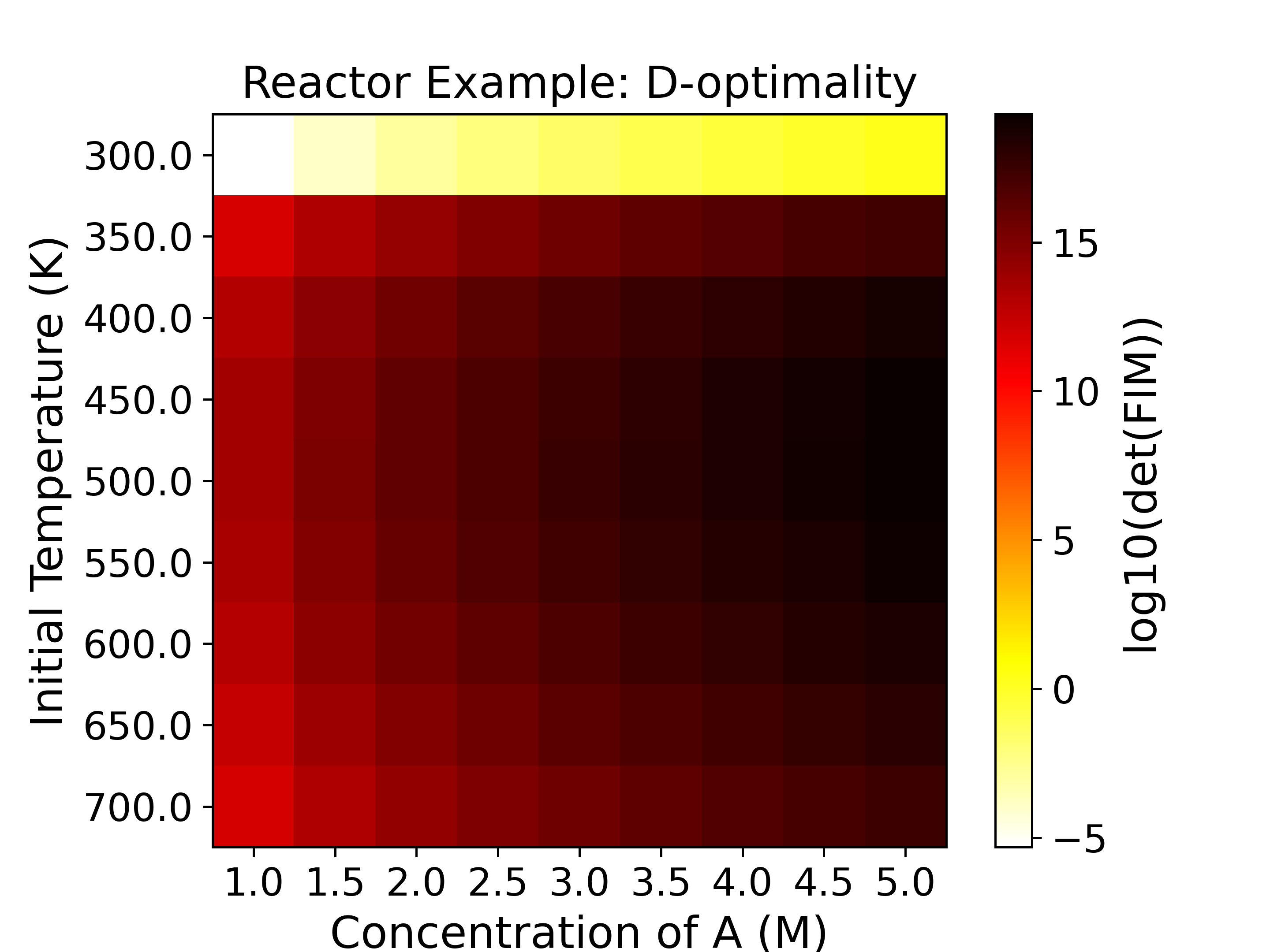
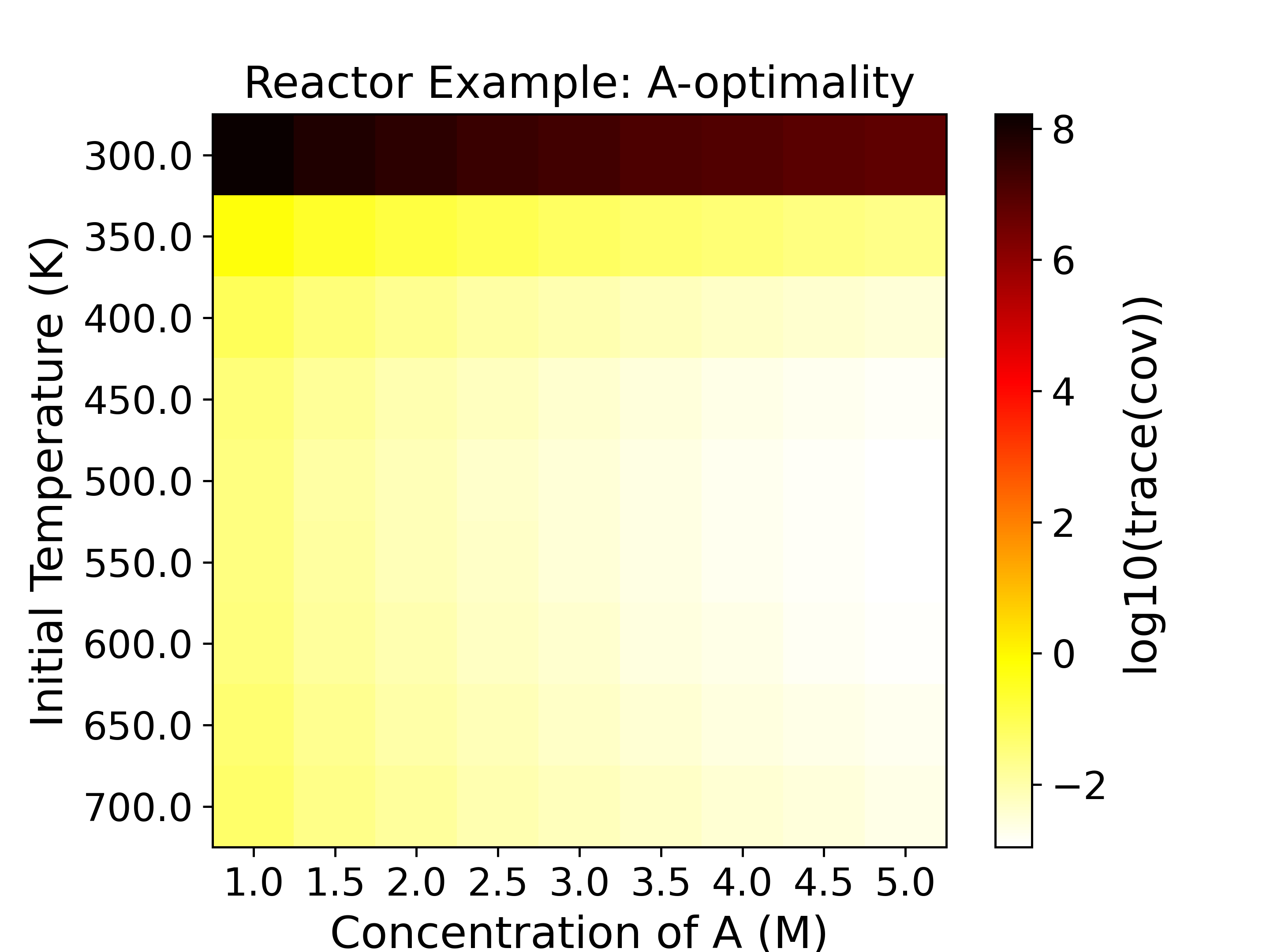
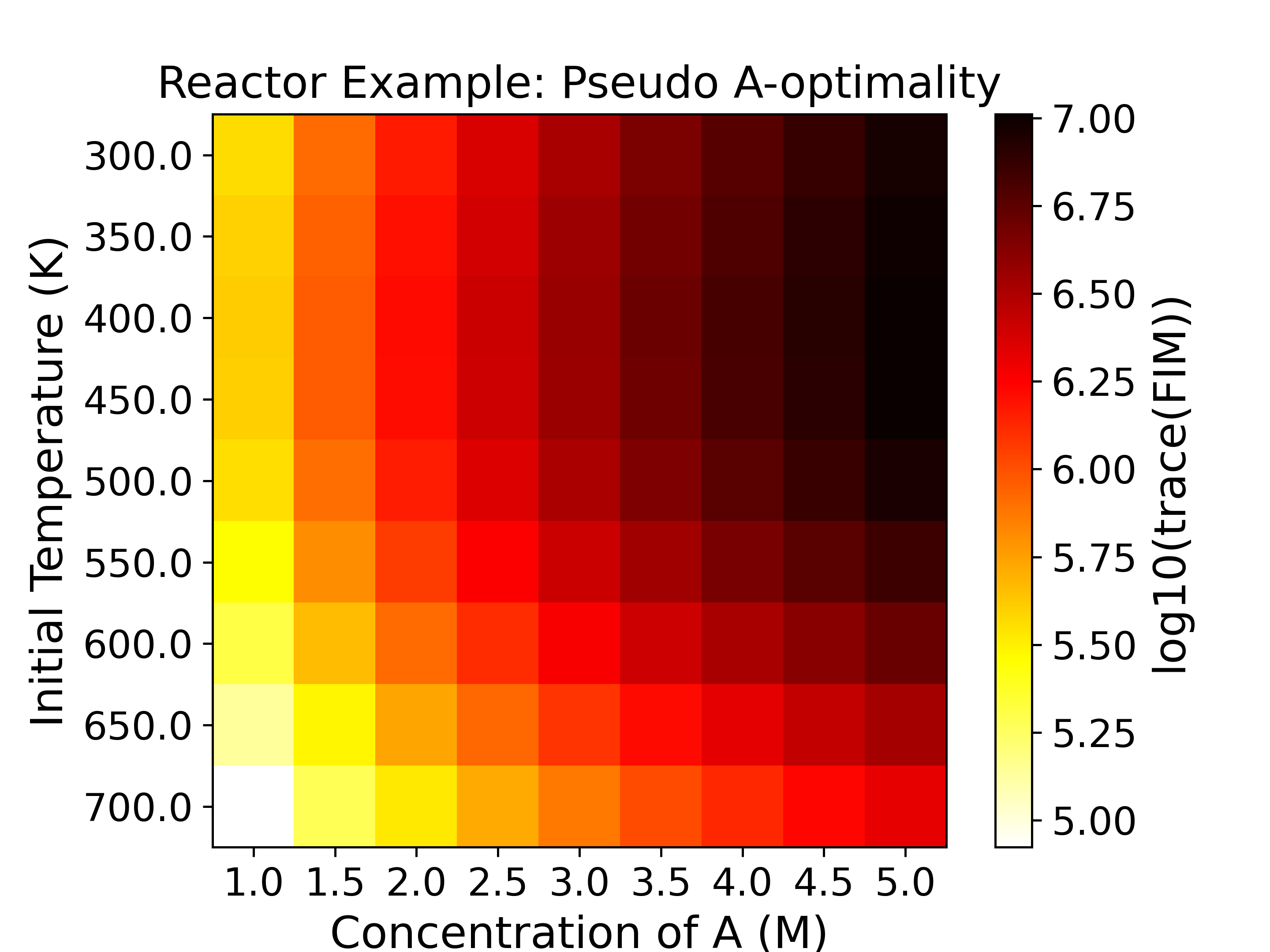
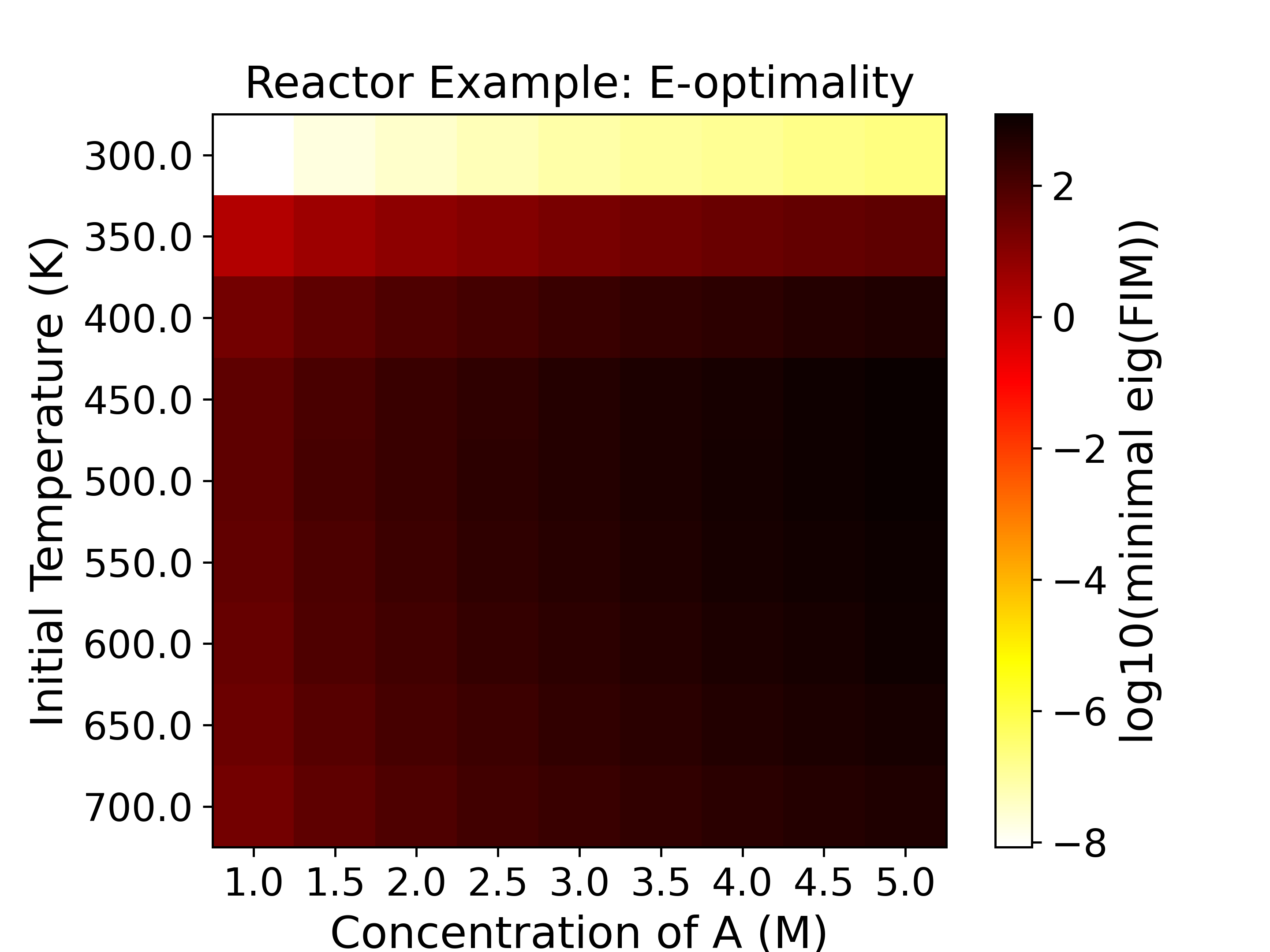
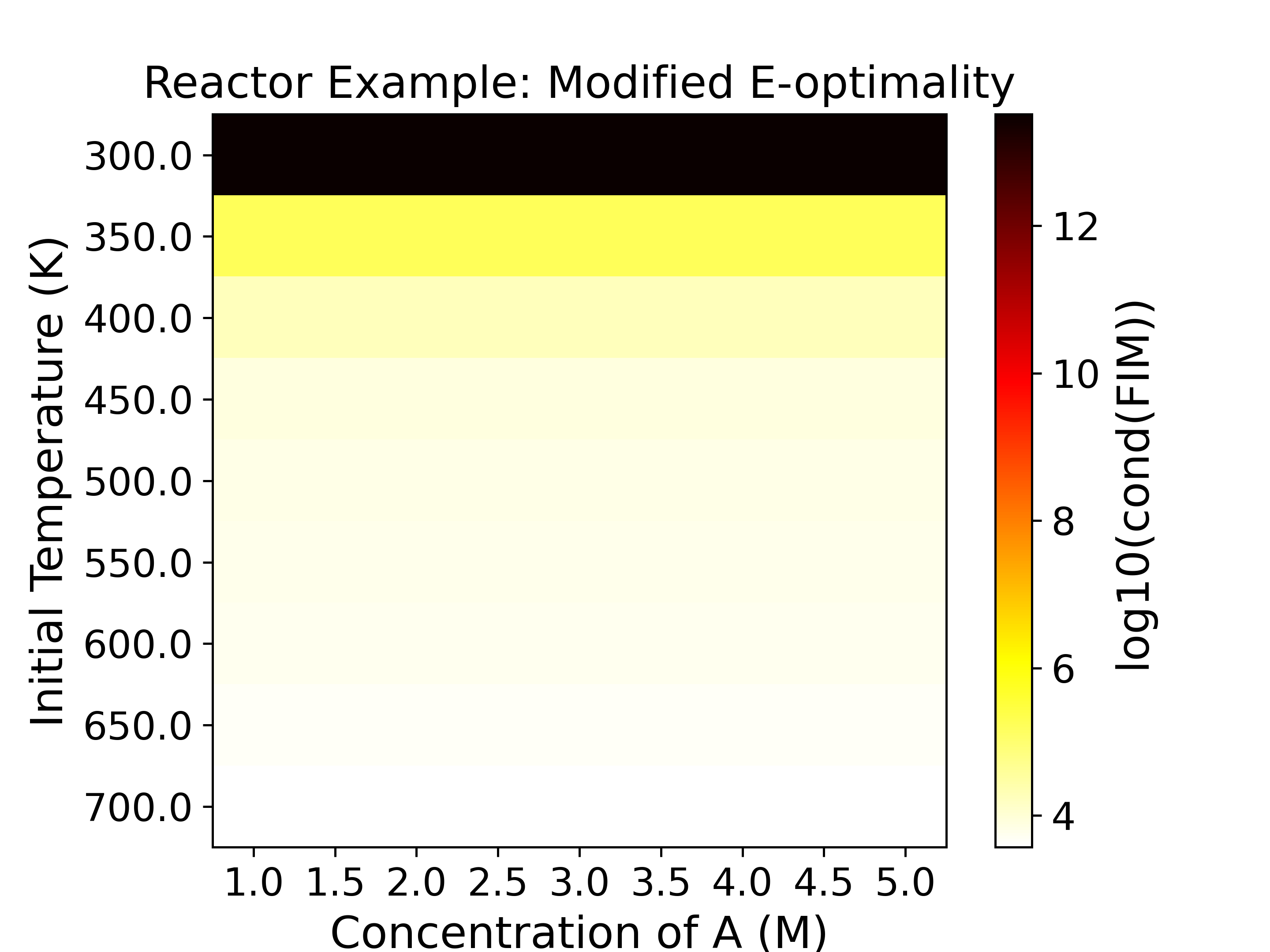
The heatmaps show the values of the objective functions, a.k.a. the
experimental information content, in the design space. Horizontal
and vertical axes are the two experimental design variables, while
the color of each grid shows the experimental information content.
For example, the D-optimality (upper left subplot) heatmap figure shows that the
most informative region is around \(C_{A0}=5.0\) M, \(T=500.0\) K with
a \(\log_{10}\) determinant of FIM being around 19,
while the least informative region is around \(C_{A0}=1.0\) M, \(T=300.0\) K,
with a \(\log_{10}\) determinant of FIM being around -5. For D-, Pseudo A-, and
E-optimality we want to maximize the objective function, while for A- and Modified
E-optimality we want to minimize the objective function.
In this sensitivity analysis plot (heatmap), we only varied the initial
concentration and the initial temperature, while the temperature at other time
points is fixed at 300 K.
\[
T(t) = \begin{cases}
T_0, & t \le 0.125 \\
300\ \text{K}, & t > 0.125
\end{cases}
\]
If \(T_0 = 300\ \text{K}\), the reaction is conducted under strictly isothermal
conditions. Because the temperature is constant, the sensitivities of the species
concentrations with respect to the Arrhenius parameters (\(A_i\) and \(E_i\))
become linearly dependent. This high correlation means the effects of the
pre-exponential factor and the activation energy cannot be uniquely distinguished
from the measurements. Consequently, the Fisher Information Matrix (FIM) becomes
ill-conditioned, resulting in a near-zero determinant and a very large condition number.
To break this correlation and make the parameters identifiable, introducing a time-
varying temperature profile (for example, a temperature step or a ramp) is required.
As shown in the heatmap, when the initial temperature \(T_0\) differs from the
subsequent 300 K baseline, such a temperature change breaks the linear dependence,
yielding a well-conditioned FIM and identifiable parameters.