aslfunctions

Pyomo provides a set of AMPL user-defined functions that commonly occur but cannot be easily written as Pyomo expressions.

Using These AMPL External Functions

Build

You must build the Pyomo extensions to use these functions. Run pyomo build-extensions in the terminal and make sure the aslfunctions build status is “ok.”

Example

>>> import pyomo.environ as pyo
>>> from pyomo.common.fileutils import find_library
>>> flib = find_library("aslfunctions")
>>> m = pyo.ConcreteModel(name = 'AMPLExternalFunctions')
>>> m.sinc = pyo.ExternalFunction(library=flib, function="sinc")
>>> m.x = pyo.Var()
>>> m.z = pyo.Var()
>>> m.constraint = pyo.Constraint(expr = m.z == m.sinc(m.x))

Functions

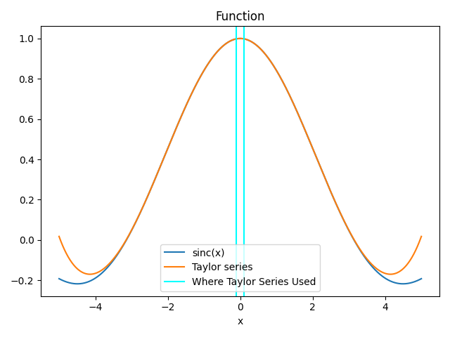
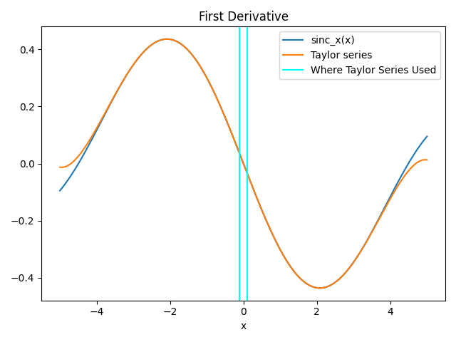
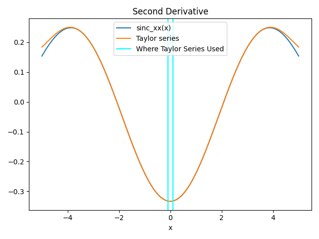
sinc(x)

This function is defined as:

\[\begin{split}\text{sinc}(x) = \begin{cases} \sin(x) / x & \text{if } x \neq 0 \\ 1 & \text{if } x = 0 \end{cases}\end{split}\]

In this implementation, the region \(-0.1 < x < 0.1\) is replaced by a Taylor series with enough terms that the function should be at least \(C^2\) smooth. The difference between the function and the Tayor series is near the limits of machine precision, about \(1 \times 10^{-16}\) for the function value, \(1 \times 10^{-16}\) for the first derivative, and \(1 \times 10^{-14}\) for the second derivative.

These figures show the sinc(x) function, the Taylor series and where the Taylor series is used.

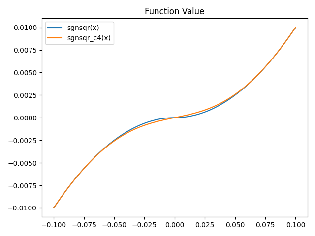
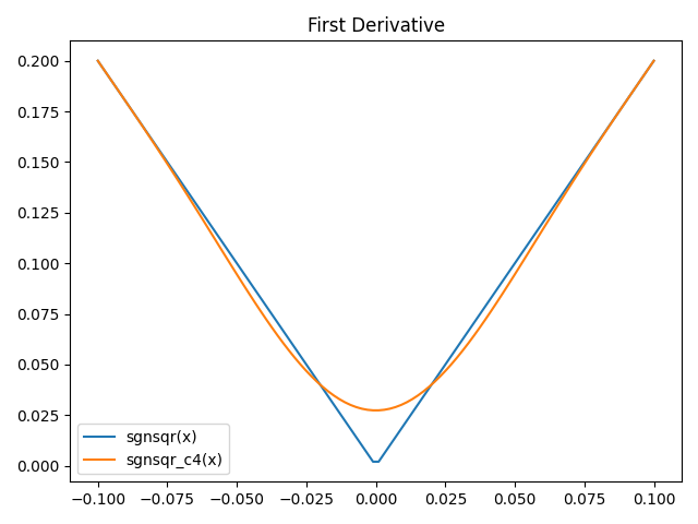
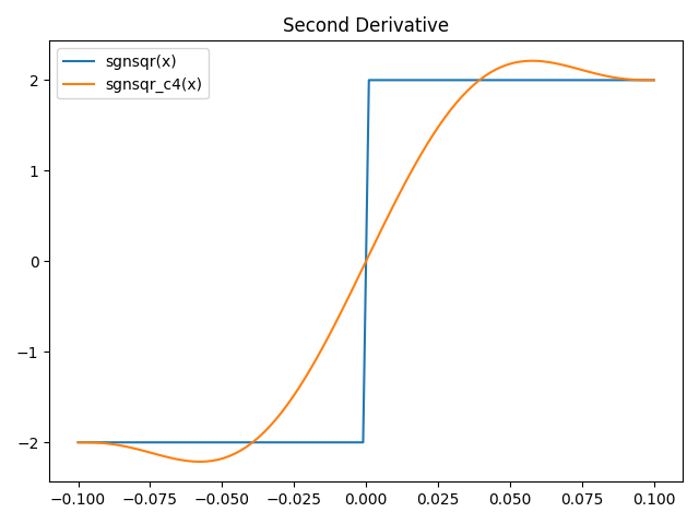
sgnsqr(x)

This function is defined as:

\[\text{sgnsqr}(x) = \text{sgn}(x)x^2\]

This function is only \(C^1\) smooth because at 0 the second derivative is undefined and the jumps from -2 to 2.

sgnsqr_c4(x)

This function is defined as:

\[\begin{split}\operatorname{sgnsqr\_c4}(x) = \begin{cases} \operatorname{sgn}(x)\,x^2 & \text{if } |x| \ge 0.1, \\ \displaystyle\sum_{i=0}^{11} c_i x^i & \text{if } |x| < 0.1 \end{cases}\end{split}\]

This function is \(C^4\) smooth. The region \(-0.1 < x < 0.1\) is replaced by an 11th order polynomial that approximates \(\text{sgn}(x)x^2\). This function has well behaved derivatives at \(x=0\). If you need to use this function with very small numbers and high accuracy is important, you can scale the argument up (e.g. \(\operatorname{sgnsqr\_c4}(sx)/s^2\)).

These figures show the sgnsqr(x) function compared to the smooth approximation sgnsqr_c4(x).

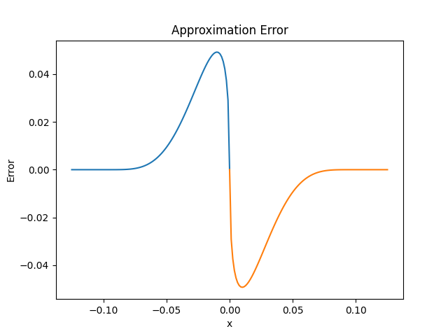
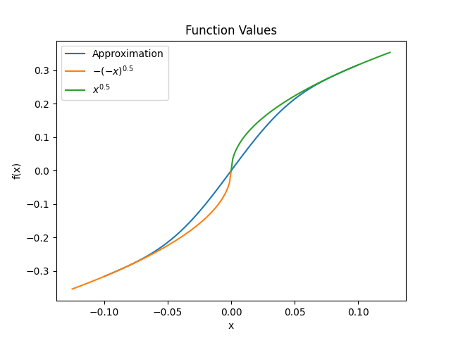
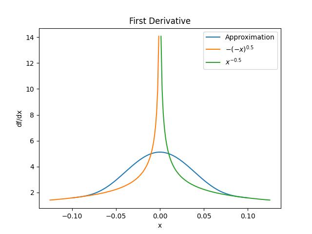
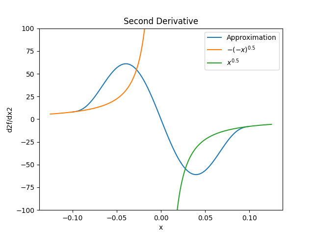
sgnsqrt_c4(x)

This function is a signed square root approximation defined as:

\[\begin{split}\operatorname{sgnsqrt\_c4}(x) = \begin{cases} \operatorname{sgn}(x)\,|x|^{0.5} & \text{if } |x| \ge 0.1, \\ \displaystyle\sum_{i=0}^{11} c_i x^i & \text{if } |x| < 0.1 \end{cases}\end{split}\]

This function is \(C^4\) smooth. The region \(-0.1 < x < 0.1\) is replaced by an 11th order polynomial that approximates \(\text{sgn}(x)|x|^{0.5}\). This function has well behaved derivatives at \(x=0\). If you need to use this function with very small numbers and high accuracy is important, you can scale the argument up (e.g. \(\operatorname{sgnsqrt\_c4}(sx)/s^{0.5}\)).

These figures show the signed square root function compared to the smooth approximation sgnsqrt_c4(x).